Keyword [Policy Gradient] [ENAS] [Parameter Share]
Pham H, Guan M Y, Zoph B, et al. Efficient neural architecture search via parameter sharing[J]. arXiv preprint arXiv:1802.03268, 2018.
1. Overview
1.1. Motivation
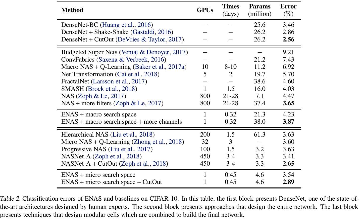
NAS use 450 GPUs for 3-4 days (32,400-43,200 hours).
In this paper, it proposes Efficient Neural Architecture Search (ENAS) algorithm.
1) Define the search space as a Graph.
2) Share parameters among child models.
3) 1000 times speed up (GPU hours), only need single GPU
2. ENAS
2.1. Design Recurrent Cells


1) $x_t$. the input signal.
2) In $Node$ $2$, Controller decides previous node index and activation function.
3) In each pair of node, there is an independent parameter matrix $W_{l,j}^{(h)}$. Therefore, all recurrent cells in a search space (graph) share the same set of parameters.
4) The search space has $4^N \times N!$ configurations (4 means tanh, ReLU, identity and Sigmoid. And node number $N=12$).
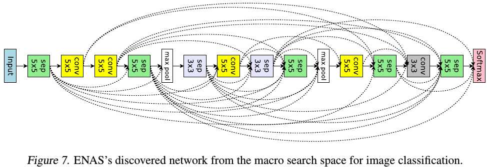
2.2. Design ConvNet

1) In $Node$ $2$, Controller decides previous node index and computation operation.
2) Computation Operation. Conv $3 \times 3$ and $5 \times 5$, DSConv $3 \times 3$ and $5 \times 5$, MaxPool $3 \times 3$ and AvgPool $3 \times 3$.
3) Make decisions $L$ times to sample a network of $L$ layers. Total $6^L \times 2^{L(L-1)/2}$ networks ($L=12$).
2.3. Design Conv Cells
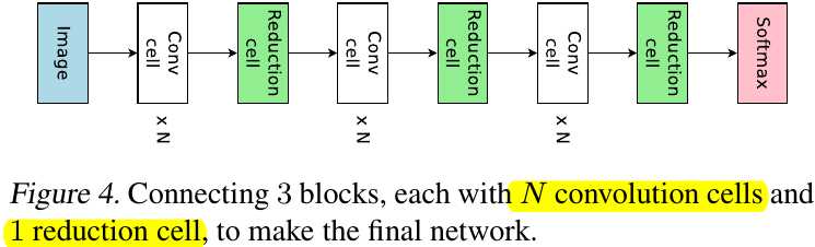

1) $Node$ $1$ and $Node$ $2$ are cell’s inputs (Node number $B=7$).
2) In $Node$ $3$, Controller decides two previous node index and two computation operation.
3) Computation Operation. Identity, DSConv $3 \times 3$ and $5 \times 5$, MaxPool $3 \times 3$ and AvgPool $3 \times 3$.
4) Node index which never been sampled will be Concat to form the cell’s output.
5) Reduction Cell. change the step to 2.
2.4. Traning Procedure
1) Controller LSTM parameters $\theta$ and shared parameters of the child models $\omega$.
2) At the first step, Controller’s input is an empty embedding.
3) Alternate training $\theta$ and $\omega$.
2.4.1 Training $\omega$

1) Fix Controller $\pi (m;\theta)$, perform SGD on $\omega$.
2) Find that $M=1$ works just fine, which means ENAS can update $\omega$ from any single model $m$ sampled from $\pi(m;\theta)$.
3) For language model, train for about 400 steps, batch_size 64.
4) For CIRFAR-10, train on 45,000 training images, batch_size 128.
2.4.2 Training $\theta$
1) Fix $\omega$, update $\theta$ with Adam & Policy Gradient.
2) $R(m, $\omega$)$ is computed on a batch of valid set.
3) Train for 2000 steps.
2.5. Deriving Architectures
1) Sample several models from $\pi (m;\theta)$.
2) For each sampled model, compute $R$ on a single batch from valid set.
3) Take the best model to retrain.
It also can train all the sampled models from scratch, then select the best on a separated validation set. But above method gets similar performance with much economical.
3. Experiments
3.1. RNN Cell Searching

3.2. ConvNet Searching
3.3. Conv Cell Searching

3.4. Comparison